In [3]:
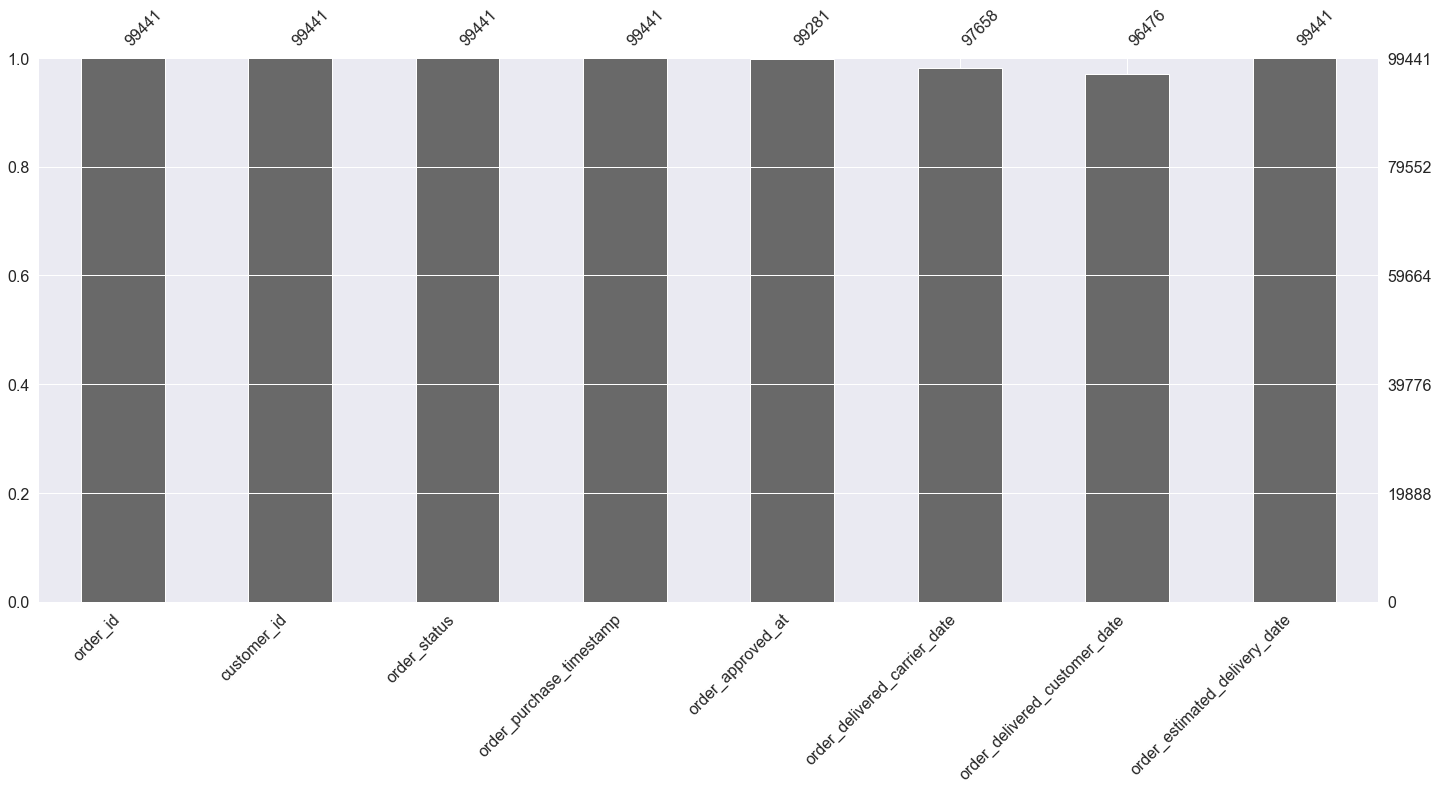
msno.bar(orders)
Out[3]:
<AxesSubplot:>
Link to datasets: https://www.kaggle.com/olistbr/brazilian-ecommerce
import numpy as np
import pandas as pd
import os
import matplotlib.pyplot as plt
import missingno as msno
import param
import panel as pn
import seaborn as sns
pn.extension()
orders = pd.read_csv("olist_orders_dataset.csv")
orders.head(3)
| order_id | customer_id | order_status | order_purchase_timestamp | order_approved_at | order_delivered_carrier_date | order_delivered_customer_date | order_estimated_delivery_date | |
|---|---|---|---|---|---|---|---|---|
| 0 | e481f51cbdc54678b7cc49136f2d6af7 | 9ef432eb6251297304e76186b10a928d | delivered | 2017-10-02 10:56:33 | 2017-10-02 11:07:15 | 2017-10-04 19:55:00 | 2017-10-10 21:25:13 | 2017-10-18 00:00:00 |
| 1 | 53cdb2fc8bc7dce0b6741e2150273451 | b0830fb4747a6c6d20dea0b8c802d7ef | delivered | 2018-07-24 20:41:37 | 2018-07-26 03:24:27 | 2018-07-26 14:31:00 | 2018-08-07 15:27:45 | 2018-08-13 00:00:00 |
| 2 | 47770eb9100c2d0c44946d9cf07ec65d | 41ce2a54c0b03bf3443c3d931a367089 | delivered | 2018-08-08 08:38:49 | 2018-08-08 08:55:23 | 2018-08-08 13:50:00 | 2018-08-17 18:06:29 | 2018-09-04 00:00:00 |
Looking into delivery
orders['order_purchase_timestamp'] = pd.to_datetime(orders.order_purchase_timestamp)
orders['order_approved_at'] = pd.to_datetime(orders.order_approved_at)
orders['order_delivered_carrier_date'] = pd.to_datetime(orders.order_delivered_carrier_date)
orders['order_delivered_customer_date'] = pd.to_datetime(orders.order_delivered_customer_date)
orders['order_estimated_delivery_date'] = pd.to_datetime(orders.order_estimated_delivery_date)
orders.head(3)
| order_id | customer_id | order_status | order_purchase_timestamp | order_approved_at | order_delivered_carrier_date | order_delivered_customer_date | order_estimated_delivery_date | |
|---|---|---|---|---|---|---|---|---|
| 0 | e481f51cbdc54678b7cc49136f2d6af7 | 9ef432eb6251297304e76186b10a928d | delivered | 2017-10-02 10:56:33 | 2017-10-02 11:07:15 | 2017-10-04 19:55:00 | 2017-10-10 21:25:13 | 2017-10-18 |
| 1 | 53cdb2fc8bc7dce0b6741e2150273451 | b0830fb4747a6c6d20dea0b8c802d7ef | delivered | 2018-07-24 20:41:37 | 2018-07-26 03:24:27 | 2018-07-26 14:31:00 | 2018-08-07 15:27:45 | 2018-08-13 |
| 2 | 47770eb9100c2d0c44946d9cf07ec65d | 41ce2a54c0b03bf3443c3d931a367089 | delivered | 2018-08-08 08:38:49 | 2018-08-08 08:55:23 | 2018-08-08 13:50:00 | 2018-08-17 18:06:29 | 2018-09-04 |
msno.bar(orders)
<AxesSubplot:>
Focus on delivered orders only
orders['order_status'].unique()
array(['delivered', 'invoiced', 'shipped', 'processing', 'unavailable',
'canceled', 'created', 'approved'], dtype=object)
delivered = orders[orders['order_status'] == 'delivered']
delivered = delivered.drop(columns="order_status")
delivered.head(3)
| order_id | customer_id | order_purchase_timestamp | order_approved_at | order_delivered_carrier_date | order_delivered_customer_date | order_estimated_delivery_date | |
|---|---|---|---|---|---|---|---|
| 0 | e481f51cbdc54678b7cc49136f2d6af7 | 9ef432eb6251297304e76186b10a928d | 2017-10-02 10:56:33 | 2017-10-02 11:07:15 | 2017-10-04 19:55:00 | 2017-10-10 21:25:13 | 2017-10-18 |
| 1 | 53cdb2fc8bc7dce0b6741e2150273451 | b0830fb4747a6c6d20dea0b8c802d7ef | 2018-07-24 20:41:37 | 2018-07-26 03:24:27 | 2018-07-26 14:31:00 | 2018-08-07 15:27:45 | 2018-08-13 |
| 2 | 47770eb9100c2d0c44946d9cf07ec65d | 41ce2a54c0b03bf3443c3d931a367089 | 2018-08-08 08:38:49 | 2018-08-08 08:55:23 | 2018-08-08 13:50:00 | 2018-08-17 18:06:29 | 2018-09-04 |
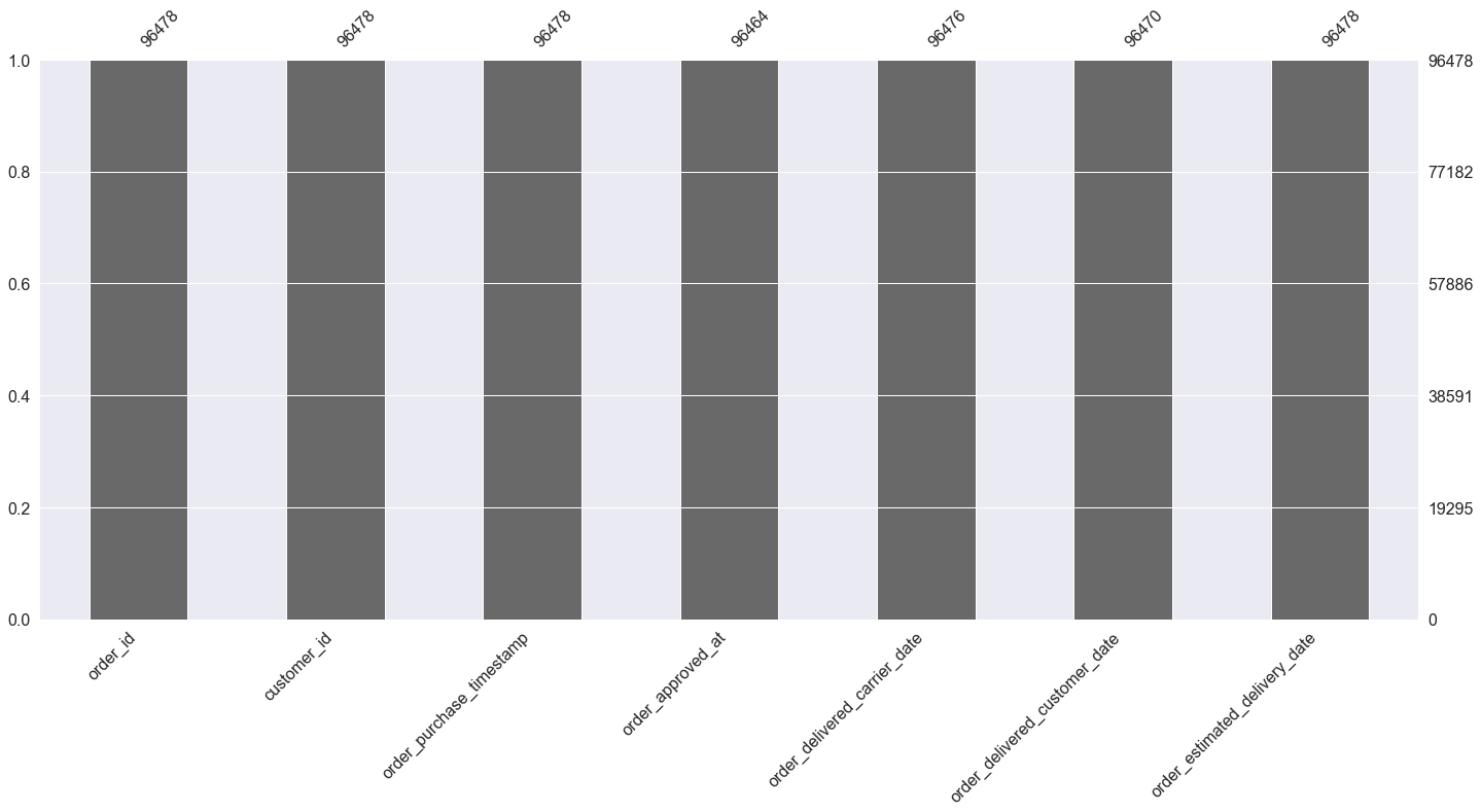
msno.bar(delivered)
<AxesSubplot:>
delivered = delivered.dropna()
msno.bar(delivered)
<AxesSubplot:>

Focus on 2017 and 2018 only, since very little data from 2016.
delivered['order_purchase_timestamp'].dt.year.value_counts().plot.bar()
delivered = orders[orders['order_purchase_timestamp'].dt.year > 2016]
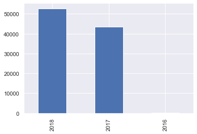
Overall sales increased in 2018.
class DeliveredDashboard(param.Parameterized):
year = param.ObjectSelector(default=2017, objects=[2017, 2018])
plt.figure(figsize=(12,8), dpi= 100)
def sales_plot(self):
plt.clf()
delivered[delivered['order_purchase_timestamp'].dt.year==self.year]['order_purchase_timestamp'].dt.month.value_counts().plot.bar()
return plt.gcf()
def total_plot(self):
plt.clf()
delivered['order_purchase_timestamp'].dt.year.value_counts().plot.bar()
return plt.gcf()
def append_end(self):
plt.clf()
return ""
dd1 = DeliveredDashboard(name='')
dashboard = pn.Column('Sales Dashboard',
dd1.param,
pn.Tabs(
('Sales by year', dd1.sales_plot),
('Total Sales', dd1.total_plot),
('',dd1.append_end)
)
)
dashboard.embed()
<Figure size 1728x1152 with 0 Axes>
Counting delivery speed and delay
delivered['order_delay'] = (delivered['order_delivered_customer_date'] - delivered['order_estimated_delivery_date']).dt.components['days']
delivered['order_duration'] = (delivered['order_delivered_customer_date'] - delivered['order_purchase_timestamp']).dt.components['days']
delivered['year'] = np.where((delivered.order_purchase_timestamp.dt.year == 2017), 2017, 2018)
delivered.head(3)
<ipython-input-10-6e47f4c74239>:1: SettingWithCopyWarning: A value is trying to be set on a copy of a slice from a DataFrame. Try using .loc[row_indexer,col_indexer] = value instead See the caveats in the documentation: https://pandas.pydata.org/pandas-docs/stable/user_guide/indexing.html#returning-a-view-versus-a-copy delivered['order_delay'] = (delivered['order_delivered_customer_date'] - delivered['order_estimated_delivery_date']).dt.components['days'] <ipython-input-10-6e47f4c74239>:2: SettingWithCopyWarning: A value is trying to be set on a copy of a slice from a DataFrame. Try using .loc[row_indexer,col_indexer] = value instead See the caveats in the documentation: https://pandas.pydata.org/pandas-docs/stable/user_guide/indexing.html#returning-a-view-versus-a-copy delivered['order_duration'] = (delivered['order_delivered_customer_date'] - delivered['order_purchase_timestamp']).dt.components['days'] <ipython-input-10-6e47f4c74239>:3: SettingWithCopyWarning: A value is trying to be set on a copy of a slice from a DataFrame. Try using .loc[row_indexer,col_indexer] = value instead See the caveats in the documentation: https://pandas.pydata.org/pandas-docs/stable/user_guide/indexing.html#returning-a-view-versus-a-copy delivered['year'] = np.where((delivered.order_purchase_timestamp.dt.year == 2017), 2017, 2018)
| order_id | customer_id | order_status | order_purchase_timestamp | order_approved_at | order_delivered_carrier_date | order_delivered_customer_date | order_estimated_delivery_date | order_delay | order_duration | year | |
|---|---|---|---|---|---|---|---|---|---|---|---|
| 0 | e481f51cbdc54678b7cc49136f2d6af7 | 9ef432eb6251297304e76186b10a928d | delivered | 2017-10-02 10:56:33 | 2017-10-02 11:07:15 | 2017-10-04 19:55:00 | 2017-10-10 21:25:13 | 2017-10-18 | -8.0 | 8.0 | 2017 |
| 1 | 53cdb2fc8bc7dce0b6741e2150273451 | b0830fb4747a6c6d20dea0b8c802d7ef | delivered | 2018-07-24 20:41:37 | 2018-07-26 03:24:27 | 2018-07-26 14:31:00 | 2018-08-07 15:27:45 | 2018-08-13 | -6.0 | 13.0 | 2018 |
| 2 | 47770eb9100c2d0c44946d9cf07ec65d | 41ce2a54c0b03bf3443c3d931a367089 | delivered | 2018-08-08 08:38:49 | 2018-08-08 08:55:23 | 2018-08-08 13:50:00 | 2018-08-17 18:06:29 | 2018-09-04 | -18.0 | 9.0 | 2018 |
delivered_stats = ['order_duration', 'order_delay']
def remove_outlier_iqr(df, col):
IQR = df[col].quantile(0.25) - df[col].quantile(0.75)
new_df = df.loc[(df[col] > (df[col].quantile(0.25) + 1.5 * IQR)) & (df[col] < (df[col].quantile(0.75) - 1.5 * IQR))]
return(new_df)
class DeliveredDashboard2(param.Parameterized):
stats = param.ObjectSelector(default='order_duration', objects=delivered_stats)
plt.figure(figsize=(12,8), dpi= 100)
def original_boxplot(self):
plt.clf()
sns.boxplot(x=delivered[self.stats])
return plt.gcf()
def after_boxplot(self):
plt.clf()
order_no_outlier = remove_outlier_iqr(delivered, 'order_duration')
sns.boxplot(x=order_no_outlier[self.stats])
return plt.gcf()
def append_end(self):
plt.clf()
return ""
dd2 = DeliveredDashboard2(name='')
dashboard = pn.Column('Outlier Dashboard',
dd2.param,
pn.Tabs(
('Original', dd2.original_boxplot),
('Outlier removed', dd2.after_boxplot),
('',dd2.append_end)
)
)
dashboard.embed()
<Figure size 1728x1152 with 0 Axes>
class DeliveredDashboard3(param.Parameterized):
stats = param.ObjectSelector(default='order_duration', objects=delivered_stats)
plt.figure(figsize=(12,8), dpi= 100)
def after_boxplot(self, year):
plt.clf()
order_no_outlier = remove_outlier_iqr(delivered[delivered['year']==year], self.stats)
sns.boxplot(x=order_no_outlier[self.stats])
return plt.gcf()
def boxplot_2017(self):
return self.after_boxplot(2017)
def boxplot_2018(self):
return self.after_boxplot(2018)
def append_end(self):
plt.clf()
return ""
dd3 = DeliveredDashboard3(name='')
dashboard = pn.Column('Delivered Outlier Dashboard',
dd3.param,
pn.Tabs(
('2017', dd3.boxplot_2017),
('2018', dd3.boxplot_2018),
('',dd3.append_end)
)
)
dashboard.embed()
<Figure size 1728x1152 with 0 Axes>
Problem identified: On average, delivery duration has decreased in 2018 and the delay is more than -10 days. At an average of 9 days of delivery, it can still be improved.
customer_visit_count = orders.groupby(['customer_id']).size().reset_index(name='count')
customer_visit_count.head(3)
| customer_id | count | |
|---|---|---|
| 0 | 00012a2ce6f8dcda20d059ce98491703 | 1 |
| 1 | 000161a058600d5901f007fab4c27140 | 1 |
| 2 | 0001fd6190edaaf884bcaf3d49edf079 | 1 |
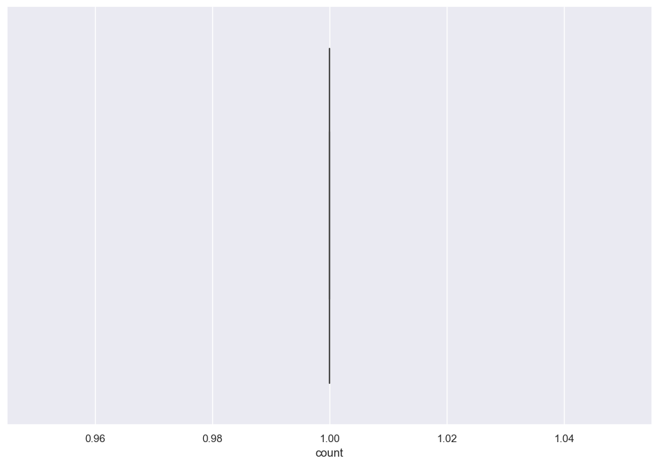
Risk: None of the customers were returning customers.
plt.figure(figsize=(12,8), dpi= 100)
sns.boxplot(x=customer_visit_count['count'])
<AxesSubplot:xlabel='count'>
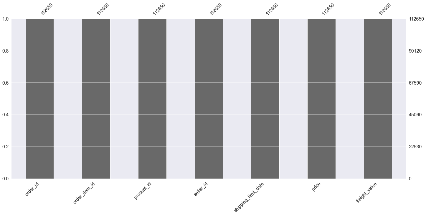
order_items = pd.read_csv("olist_order_items_dataset.csv")
order_items.head(3)
| order_id | order_item_id | product_id | seller_id | shipping_limit_date | price | freight_value | |
|---|---|---|---|---|---|---|---|
| 0 | 00010242fe8c5a6d1ba2dd792cb16214 | 1 | 4244733e06e7ecb4970a6e2683c13e61 | 48436dade18ac8b2bce089ec2a041202 | 2017-09-19 09:45:35 | 58.9 | 13.29 |
| 1 | 00018f77f2f0320c557190d7a144bdd3 | 1 | e5f2d52b802189ee658865ca93d83a8f | dd7ddc04e1b6c2c614352b383efe2d36 | 2017-05-03 11:05:13 | 239.9 | 19.93 |
| 2 | 000229ec398224ef6ca0657da4fc703e | 1 | c777355d18b72b67abbeef9df44fd0fd | 5b51032eddd242adc84c38acab88f23d | 2018-01-18 14:48:30 | 199.0 | 17.87 |
msno.bar(order_items)
<AxesSubplot:>
order_price = order_items.groupby('order_id').sum('price')
order_price.head(3)
| order_item_id | price | freight_value | |
|---|---|---|---|
| order_id | |||
| 00010242fe8c5a6d1ba2dd792cb16214 | 1 | 58.9 | 13.29 |
| 00018f77f2f0320c557190d7a144bdd3 | 1 | 239.9 | 19.93 |
| 000229ec398224ef6ca0657da4fc703e | 1 | 199.0 | 17.87 |
class OrderPriceDashboard(param.Parameterized):
stats = param.ObjectSelector(default='Original', objects=['Original', 'Outlier removed'])
plt.figure(figsize=(12,8), dpi= 100)
def after_boxplot(self):
plt.clf()
if self.stats == 'Original':
sns.boxplot(x=order_price['price'])
else:
order_no_outlier = remove_outlier_iqr(order_price, 'price')
sns.boxplot(x=order_no_outlier['price'])
return plt.gcf()
def append_end(self):
plt.clf()
return ""
op1 = OrderPriceDashboard(name='')
dashboard = pn.Column('Order Price Outlier Dashboard',
op1.param,
op1.after_boxplot,
op1.append_end
)
dashboard.embed()
<Figure size 1728x1152 with 0 Axes>
Because all the customers have only one order and are not returning customers, revenue generated by each customer was mostly only around 50 to 150.
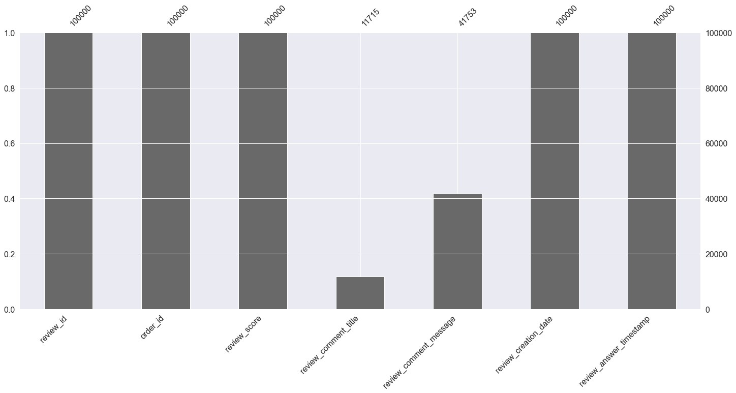
order_reviews = pd.read_csv("olist_order_reviews_dataset.csv")
order_reviews.head(3)
| review_id | order_id | review_score | review_comment_title | review_comment_message | review_creation_date | review_answer_timestamp | |
|---|---|---|---|---|---|---|---|
| 0 | 7bc2406110b926393aa56f80a40eba40 | 73fc7af87114b39712e6da79b0a377eb | 4 | NaN | NaN | 2018-01-18 00:00:00 | 2018-01-18 21:46:59 |
| 1 | 80e641a11e56f04c1ad469d5645fdfde | a548910a1c6147796b98fdf73dbeba33 | 5 | NaN | NaN | 2018-03-10 00:00:00 | 2018-03-11 03:05:13 |
| 2 | 228ce5500dc1d8e020d8d1322874b6f0 | f9e4b658b201a9f2ecdecbb34bed034b | 5 | NaN | NaN | 2018-02-17 00:00:00 | 2018-02-18 14:36:24 |
msno.bar(order_reviews)
<AxesSubplot:>
I have used Google Translate to translate the reviews from Portugese to English, then saved the output in a local html file. So, I am scraping from the html file.
import codecs
from bs4 import BeautifulSoup
def soup_table(file):
f=codecs.open(file, 'r')
html = BeautifulSoup(f, 'html.parser')
html = html.find_all('td', {'align':'left'})
txt_list = []
for tr in html:
txt_list.append(tr.text)
return(txt_list)
english_title = soup_table('english_title.htm')
english_title.pop(0)
len(english_title)
11715
Based on the number, I can assume that all comments were translated and successfully scraped.
english_comment = soup_table('english_comment.htm')
english_comment.pop(0)
len(english_comment)
41753
Because Google Translate only accepts .xlsx, I have to read the excel back into a dataframe to map the translation back to its review id.
from pandas import read_excel
title_xlsx = read_excel('english_title.xlsx')
title_xlsx.head(3)
| Unnamed: 0 | review_id | review_comment_title | |
|---|---|---|---|
| 0 | 9 | 8670d52e15e00043ae7de4c01cc2fe06 | recomendo |
| 1 | 15 | 3948b09f7c818e2d86c9a546758b2335 | super recomendo |
| 2 | 19 | 373cbeecea8286a2b66c97b1b157ec46 | negação chegou produto |
title_xlsx = title_xlsx.drop(title_xlsx.columns[[0, 2]], axis=1)
title_xlsx['translated_title'] = english_title
title_xlsx.head(3)
| review_id | translated_title | |
|---|---|---|
| 0 | 8670d52e15e00043ae7de4c01cc2fe06 | I recommend |
| 1 | 3948b09f7c818e2d86c9a546758b2335 | super recommend |
| 2 | 373cbeecea8286a2b66c97b1b157ec46 | denial arrived product |
comment_xlsx = read_excel('english_comment.xlsx')
comment_xlsx.head(3)
| Unnamed: 0 | review_id | review_comment_message | |
|---|---|---|---|
| 0 | 3 | e64fb393e7b32834bb789ff8bb30750e | recebi bem antes prazo estipulado |
| 1 | 4 | f7c4243c7fe1938f181bec41a392bdeb | parabéns lojas lannister adorei comprar intern... |
| 2 | 9 | 8670d52e15e00043ae7de4c01cc2fe06 | aparelho eficiente site marca aparelho impress... |
comment_xlsx = comment_xlsx.drop(comment_xlsx.columns[[0, 2]], axis=1)
comment_xlsx['translated_comment'] = english_comment
comment_xlsx.head(3)
| review_id | translated_comment | |
|---|---|---|
| 0 | e64fb393e7b32834bb789ff8bb30750e | I received it well before the deadline |
| 1 | f7c4243c7fe1938f181bec41a392bdeb | congratulations lannister stores loved buying ... |
| 2 | 8670d52e15e00043ae7de4c01cc2fe06 | efficient device website brand device printed ... |
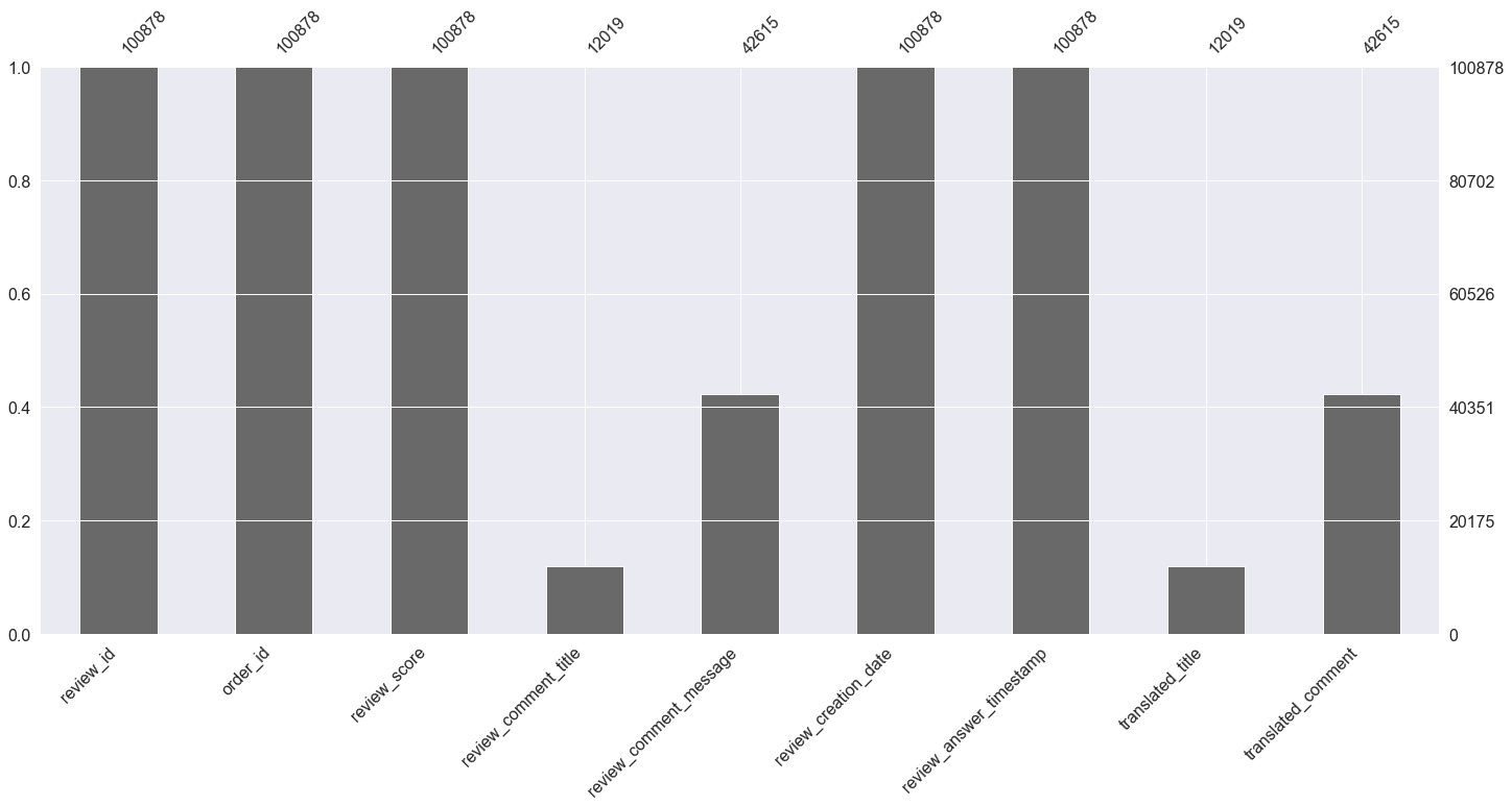
translated_order_reviews = pd.merge(order_reviews, title_xlsx, left_on='review_id', right_on='review_id', how='left')
translated_order_reviews = pd.merge(translated_order_reviews, comment_xlsx, left_on='review_id', right_on='review_id', how='left')
translated_order_reviews.head(10)
| review_id | order_id | review_score | review_comment_title | review_comment_message | review_creation_date | review_answer_timestamp | translated_title | translated_comment | |
|---|---|---|---|---|---|---|---|---|---|
| 0 | 7bc2406110b926393aa56f80a40eba40 | 73fc7af87114b39712e6da79b0a377eb | 4 | NaN | NaN | 2018-01-18 00:00:00 | 2018-01-18 21:46:59 | NaN | NaN |
| 1 | 80e641a11e56f04c1ad469d5645fdfde | a548910a1c6147796b98fdf73dbeba33 | 5 | NaN | NaN | 2018-03-10 00:00:00 | 2018-03-11 03:05:13 | NaN | NaN |
| 2 | 228ce5500dc1d8e020d8d1322874b6f0 | f9e4b658b201a9f2ecdecbb34bed034b | 5 | NaN | NaN | 2018-02-17 00:00:00 | 2018-02-18 14:36:24 | NaN | NaN |
| 3 | e64fb393e7b32834bb789ff8bb30750e | 658677c97b385a9be170737859d3511b | 5 | NaN | Recebi bem antes do prazo estipulado. | 2017-04-21 00:00:00 | 2017-04-21 22:02:06 | NaN | I received it well before the deadline |
| 4 | f7c4243c7fe1938f181bec41a392bdeb | 8e6bfb81e283fa7e4f11123a3fb894f1 | 5 | NaN | Parabéns lojas lannister adorei comprar pela I... | 2018-03-01 00:00:00 | 2018-03-02 10:26:53 | NaN | congratulations lannister stores loved buying ... |
| 5 | 15197aa66ff4d0650b5434f1b46cda19 | b18dcdf73be66366873cd26c5724d1dc | 1 | NaN | NaN | 2018-04-13 00:00:00 | 2018-04-16 00:39:37 | NaN | NaN |
| 6 | 07f9bee5d1b850860defd761afa7ff16 | e48aa0d2dcec3a2e87348811bcfdf22b | 5 | NaN | NaN | 2017-07-16 00:00:00 | 2017-07-18 19:30:34 | NaN | NaN |
| 7 | 7c6400515c67679fbee952a7525281ef | c31a859e34e3adac22f376954e19b39d | 5 | NaN | NaN | 2018-08-14 00:00:00 | 2018-08-14 21:36:06 | NaN | NaN |
| 8 | a3f6f7f6f433de0aefbb97da197c554c | 9c214ac970e84273583ab523dfafd09b | 5 | NaN | NaN | 2017-05-17 00:00:00 | 2017-05-18 12:05:37 | NaN | NaN |
| 9 | 8670d52e15e00043ae7de4c01cc2fe06 | b9bf720beb4ab3728760088589c62129 | 4 | recomendo | aparelho eficiente. no site a marca do aparelh... | 2018-05-22 00:00:00 | 2018-05-23 16:45:47 | I recommend | efficient device website brand device printed ... |
msno.bar(translated_order_reviews)
<AxesSubplot:>
delivery_pattern = 'early|late|deadline|stipulate|delay|deliver|fast|slow|schedule|ahead|arrive|receive|time|return|cancel|track|trip|came|speed|wait|courier|transit|month|address|day|damage|ship|condition|mail|week|package|condition|date|freight|trace'
translated_order_reviews['delivery_related'] = ((translated_order_reviews['translated_comment'].str.contains(delivery_pattern)) | (translated_order_reviews['translated_title'].str.contains(delivery_pattern)))
translated_order_reviews.loc[pd.isnull(translated_order_reviews['translated_comment']), 'delivery_related'] = 'Null'
translated_order_reviews.head(10)
| review_id | order_id | review_score | review_comment_title | review_comment_message | review_creation_date | review_answer_timestamp | translated_title | translated_comment | delivery_related | |
|---|---|---|---|---|---|---|---|---|---|---|
| 0 | 7bc2406110b926393aa56f80a40eba40 | 73fc7af87114b39712e6da79b0a377eb | 4 | NaN | NaN | 2018-01-18 00:00:00 | 2018-01-18 21:46:59 | NaN | NaN | Null |
| 1 | 80e641a11e56f04c1ad469d5645fdfde | a548910a1c6147796b98fdf73dbeba33 | 5 | NaN | NaN | 2018-03-10 00:00:00 | 2018-03-11 03:05:13 | NaN | NaN | Null |
| 2 | 228ce5500dc1d8e020d8d1322874b6f0 | f9e4b658b201a9f2ecdecbb34bed034b | 5 | NaN | NaN | 2018-02-17 00:00:00 | 2018-02-18 14:36:24 | NaN | NaN | Null |
| 3 | e64fb393e7b32834bb789ff8bb30750e | 658677c97b385a9be170737859d3511b | 5 | NaN | Recebi bem antes do prazo estipulado. | 2017-04-21 00:00:00 | 2017-04-21 22:02:06 | NaN | I received it well before the deadline | True |
| 4 | f7c4243c7fe1938f181bec41a392bdeb | 8e6bfb81e283fa7e4f11123a3fb894f1 | 5 | NaN | Parabéns lojas lannister adorei comprar pela I... | 2018-03-01 00:00:00 | 2018-03-02 10:26:53 | NaN | congratulations lannister stores loved buying ... | False |
| 5 | 15197aa66ff4d0650b5434f1b46cda19 | b18dcdf73be66366873cd26c5724d1dc | 1 | NaN | NaN | 2018-04-13 00:00:00 | 2018-04-16 00:39:37 | NaN | NaN | Null |
| 6 | 07f9bee5d1b850860defd761afa7ff16 | e48aa0d2dcec3a2e87348811bcfdf22b | 5 | NaN | NaN | 2017-07-16 00:00:00 | 2017-07-18 19:30:34 | NaN | NaN | Null |
| 7 | 7c6400515c67679fbee952a7525281ef | c31a859e34e3adac22f376954e19b39d | 5 | NaN | NaN | 2018-08-14 00:00:00 | 2018-08-14 21:36:06 | NaN | NaN | Null |
| 8 | a3f6f7f6f433de0aefbb97da197c554c | 9c214ac970e84273583ab523dfafd09b | 5 | NaN | NaN | 2017-05-17 00:00:00 | 2017-05-18 12:05:37 | NaN | NaN | Null |
| 9 | 8670d52e15e00043ae7de4c01cc2fe06 | b9bf720beb4ab3728760088589c62129 | 4 | recomendo | aparelho eficiente. no site a marca do aparelh... | 2018-05-22 00:00:00 | 2018-05-23 16:45:47 | I recommend | efficient device website brand device printed ... | True |
translated_order_reviews = pd.merge(translated_order_reviews, orders, left_on='order_id', right_on='order_id', how='left')
translated_order_reviews['year'] = np.where((translated_order_reviews.order_purchase_timestamp.dt.year == 2017), 2017, 2018)
translated_order_reviews.head(3)
| review_id | order_id | review_score | review_comment_title | review_comment_message | review_creation_date | review_answer_timestamp | translated_title | translated_comment | delivery_related | customer_id | order_status | order_purchase_timestamp | order_approved_at | order_delivered_carrier_date | order_delivered_customer_date | order_estimated_delivery_date | year | |
|---|---|---|---|---|---|---|---|---|---|---|---|---|---|---|---|---|---|---|
| 0 | 7bc2406110b926393aa56f80a40eba40 | 73fc7af87114b39712e6da79b0a377eb | 4 | NaN | NaN | 2018-01-18 00:00:00 | 2018-01-18 21:46:59 | NaN | NaN | Null | 41dcb106f807e993532d446263290104 | delivered | 2018-01-11 15:30:49 | 2018-01-11 15:47:59 | 2018-01-12 21:57:22 | 2018-01-17 18:42:41 | 2018-02-02 | 2018 |
| 1 | 80e641a11e56f04c1ad469d5645fdfde | a548910a1c6147796b98fdf73dbeba33 | 5 | NaN | NaN | 2018-03-10 00:00:00 | 2018-03-11 03:05:13 | NaN | NaN | Null | 8a2e7ef9053dea531e4dc76bd6d853e6 | delivered | 2018-02-28 12:25:19 | 2018-02-28 12:48:39 | 2018-03-02 19:08:15 | 2018-03-09 23:17:20 | 2018-03-14 | 2018 |
| 2 | 228ce5500dc1d8e020d8d1322874b6f0 | f9e4b658b201a9f2ecdecbb34bed034b | 5 | NaN | NaN | 2018-02-17 00:00:00 | 2018-02-18 14:36:24 | NaN | NaN | Null | e226dfed6544df5b7b87a48208690feb | delivered | 2018-02-03 09:56:22 | 2018-02-03 10:33:41 | 2018-02-06 16:18:28 | 2018-02-16 17:28:48 | 2018-03-09 | 2018 |
translated_order_reviews['order_duration'] = (translated_order_reviews['order_delivered_customer_date'] - translated_order_reviews['order_purchase_timestamp']).dt.components['days']
translated_order_reviews.head(3)
| review_id | order_id | review_score | review_comment_title | review_comment_message | review_creation_date | review_answer_timestamp | translated_title | translated_comment | delivery_related | customer_id | order_status | order_purchase_timestamp | order_approved_at | order_delivered_carrier_date | order_delivered_customer_date | order_estimated_delivery_date | year | order_duration | |
|---|---|---|---|---|---|---|---|---|---|---|---|---|---|---|---|---|---|---|---|
| 0 | 7bc2406110b926393aa56f80a40eba40 | 73fc7af87114b39712e6da79b0a377eb | 4 | NaN | NaN | 2018-01-18 00:00:00 | 2018-01-18 21:46:59 | NaN | NaN | Null | 41dcb106f807e993532d446263290104 | delivered | 2018-01-11 15:30:49 | 2018-01-11 15:47:59 | 2018-01-12 21:57:22 | 2018-01-17 18:42:41 | 2018-02-02 | 2018 | 6.0 |
| 1 | 80e641a11e56f04c1ad469d5645fdfde | a548910a1c6147796b98fdf73dbeba33 | 5 | NaN | NaN | 2018-03-10 00:00:00 | 2018-03-11 03:05:13 | NaN | NaN | Null | 8a2e7ef9053dea531e4dc76bd6d853e6 | delivered | 2018-02-28 12:25:19 | 2018-02-28 12:48:39 | 2018-03-02 19:08:15 | 2018-03-09 23:17:20 | 2018-03-14 | 2018 | 9.0 |
| 2 | 228ce5500dc1d8e020d8d1322874b6f0 | f9e4b658b201a9f2ecdecbb34bed034b | 5 | NaN | NaN | 2018-02-17 00:00:00 | 2018-02-18 14:36:24 | NaN | NaN | Null | e226dfed6544df5b7b87a48208690feb | delivered | 2018-02-03 09:56:22 | 2018-02-03 10:33:41 | 2018-02-06 16:18:28 | 2018-02-16 17:28:48 | 2018-03-09 | 2018 | 13.0 |
class ReviewDashboard(param.Parameterized):
stats = param.ObjectSelector(default='review_score', objects=['review_score', 'order_duration'])
sns.set(style="darkgrid")
plt.figure(figsize=(12,8), dpi= 100)
def sns_plot(self):
plt.clf()
splot = sns.barplot(x="year", y=self.stats, hue="delivery_related", data=translated_order_reviews, ci=None)
for p in splot.patches:
splot.annotate(format(p.get_height(), '.1f'),
(p.get_x() + p.get_width() / 2., p.get_height()),
ha = 'center', va = 'center',
xytext = (0, 9),
textcoords = 'offset points')
return plt.gcf()
def append_end(self):
plt.clf()
return ""
rd1 = ReviewDashboard(name='')
dashboard = pn.Column('Review Dashboard',
rd1.param,
rd1.sns_plot,
rd1.append_end
)
dashboard.embed()
<Figure size 1728x1152 with 0 Axes>
While the average review score is above 3, it tends to be lower for reviews that are related to delivery. Just like there is some improvement in delivery speed, there is slight improvement in this case too.
Average rating for reviews that mention about delivery has increased.
Average days taken to deliver has decreased for reviews that mentioned about delivery.
delivered['approval_hours'] = (delivered['order_approved_at'] - delivered['order_purchase_timestamp']).dt.components['hours']
delivered.head(3)
<ipython-input-33-838e32387169>:1: SettingWithCopyWarning: A value is trying to be set on a copy of a slice from a DataFrame. Try using .loc[row_indexer,col_indexer] = value instead See the caveats in the documentation: https://pandas.pydata.org/pandas-docs/stable/user_guide/indexing.html#returning-a-view-versus-a-copy delivered['approval_hours'] = (delivered['order_approved_at'] - delivered['order_purchase_timestamp']).dt.components['hours']
| order_id | customer_id | order_status | order_purchase_timestamp | order_approved_at | order_delivered_carrier_date | order_delivered_customer_date | order_estimated_delivery_date | order_delay | order_duration | year | approval_hours | |
|---|---|---|---|---|---|---|---|---|---|---|---|---|
| 0 | e481f51cbdc54678b7cc49136f2d6af7 | 9ef432eb6251297304e76186b10a928d | delivered | 2017-10-02 10:56:33 | 2017-10-02 11:07:15 | 2017-10-04 19:55:00 | 2017-10-10 21:25:13 | 2017-10-18 | -8.0 | 8.0 | 2017 | 0.0 |
| 1 | 53cdb2fc8bc7dce0b6741e2150273451 | b0830fb4747a6c6d20dea0b8c802d7ef | delivered | 2018-07-24 20:41:37 | 2018-07-26 03:24:27 | 2018-07-26 14:31:00 | 2018-08-07 15:27:45 | 2018-08-13 | -6.0 | 13.0 | 2018 | 6.0 |
| 2 | 47770eb9100c2d0c44946d9cf07ec65d | 41ce2a54c0b03bf3443c3d931a367089 | delivered | 2018-08-08 08:38:49 | 2018-08-08 08:55:23 | 2018-08-08 13:50:00 | 2018-08-17 18:06:29 | 2018-09-04 | -18.0 | 9.0 | 2018 | 0.0 |
orders_approval_hours = remove_outlier_iqr(delivered, 'approval_hours')
orders_approval_hours.head()
| order_id | customer_id | order_status | order_purchase_timestamp | order_approved_at | order_delivered_carrier_date | order_delivered_customer_date | order_estimated_delivery_date | order_delay | order_duration | year | approval_hours | |
|---|---|---|---|---|---|---|---|---|---|---|---|---|
| 0 | e481f51cbdc54678b7cc49136f2d6af7 | 9ef432eb6251297304e76186b10a928d | delivered | 2017-10-02 10:56:33 | 2017-10-02 11:07:15 | 2017-10-04 19:55:00 | 2017-10-10 21:25:13 | 2017-10-18 | -8.0 | 8.0 | 2017 | 0.0 |
| 1 | 53cdb2fc8bc7dce0b6741e2150273451 | b0830fb4747a6c6d20dea0b8c802d7ef | delivered | 2018-07-24 20:41:37 | 2018-07-26 03:24:27 | 2018-07-26 14:31:00 | 2018-08-07 15:27:45 | 2018-08-13 | -6.0 | 13.0 | 2018 | 6.0 |
| 2 | 47770eb9100c2d0c44946d9cf07ec65d | 41ce2a54c0b03bf3443c3d931a367089 | delivered | 2018-08-08 08:38:49 | 2018-08-08 08:55:23 | 2018-08-08 13:50:00 | 2018-08-17 18:06:29 | 2018-09-04 | -18.0 | 9.0 | 2018 | 0.0 |
| 3 | 949d5b44dbf5de918fe9c16f97b45f8a | f88197465ea7920adcdbec7375364d82 | delivered | 2017-11-18 19:28:06 | 2017-11-18 19:45:59 | 2017-11-22 13:39:59 | 2017-12-02 00:28:42 | 2017-12-15 | -13.0 | 13.0 | 2017 | 0.0 |
| 4 | ad21c59c0840e6cb83a9ceb5573f8159 | 8ab97904e6daea8866dbdbc4fb7aad2c | delivered | 2018-02-13 21:18:39 | 2018-02-13 22:20:29 | 2018-02-14 19:46:34 | 2018-02-16 18:17:02 | 2018-02-26 | -10.0 | 2.0 | 2018 | 1.0 |
class DeliverHoursDashboard(param.Parameterized):
stats = param.ObjectSelector(default='Original', objects=['Original', 'Outlier removed'])
plt.figure(figsize=(12,8), dpi= 100)
def after_boxplot(self):
plt.clf()
if self.stats == 'Original':
sns.boxplot(x=delivered['approval_hours'])
else:
sns.boxplot(x=orders_approval_hours['approval_hours'])
return plt.gcf()
def append_end(self):
plt.clf()
return ""
dh1 = DeliverHoursDashboard(name='')
dashboard = pn.Column('Delivery Hours Outlier Dashboard',
dh1.param,
dh1.after_boxplot,
dh1.append_end
)
dashboard.embed()
<Figure size 1728x1152 with 0 Axes>
It usually takes around 45 minutes for an order to be approved. This duration has increased in 2018.
order_payments = pd.read_csv("olist_order_payments_dataset.csv")
order_payments.head(3)
| order_id | payment_sequential | payment_type | payment_installments | payment_value | |
|---|---|---|---|---|---|
| 0 | b81ef226f3fe1789b1e8b2acac839d17 | 1 | credit_card | 8 | 99.33 |
| 1 | a9810da82917af2d9aefd1278f1dcfa0 | 1 | credit_card | 1 | 24.39 |
| 2 | 25e8ea4e93396b6fa0d3dd708e76c1bd | 1 | credit_card | 1 | 65.71 |
orders_approval_hours = orders_approval_hours.merge(order_payments, left_on='order_id', right_on='order_id')
orders_approval_hours.head(3)
| order_id | customer_id | order_status | order_purchase_timestamp | order_approved_at | order_delivered_carrier_date | order_delivered_customer_date | order_estimated_delivery_date | order_delay | order_duration | year | approval_hours | payment_sequential | payment_type | payment_installments | payment_value | |
|---|---|---|---|---|---|---|---|---|---|---|---|---|---|---|---|---|
| 0 | e481f51cbdc54678b7cc49136f2d6af7 | 9ef432eb6251297304e76186b10a928d | delivered | 2017-10-02 10:56:33 | 2017-10-02 11:07:15 | 2017-10-04 19:55:00 | 2017-10-10 21:25:13 | 2017-10-18 | -8.0 | 8.0 | 2017 | 0.0 | 1 | credit_card | 1 | 18.12 |
| 1 | e481f51cbdc54678b7cc49136f2d6af7 | 9ef432eb6251297304e76186b10a928d | delivered | 2017-10-02 10:56:33 | 2017-10-02 11:07:15 | 2017-10-04 19:55:00 | 2017-10-10 21:25:13 | 2017-10-18 | -8.0 | 8.0 | 2017 | 0.0 | 3 | voucher | 1 | 2.00 |
| 2 | e481f51cbdc54678b7cc49136f2d6af7 | 9ef432eb6251297304e76186b10a928d | delivered | 2017-10-02 10:56:33 | 2017-10-02 11:07:15 | 2017-10-04 19:55:00 | 2017-10-10 21:25:13 | 2017-10-18 | -8.0 | 8.0 | 2017 | 0.0 | 2 | voucher | 1 | 18.59 |
class ApprovalPaymentDashboard(param.Parameterized):
stats = param.ObjectSelector(default='approval_hours', objects=['approval_hours', 'approval_hours by payment type'])
sns.set(style="darkgrid")
plt.figure(figsize=(12,8), dpi= 100)
def sns_plot(self):
plt.clf()
if self.stats == 'approval_hours':
splot = sns.barplot(x="year", y="approval_hours",data=orders_approval_hours, ci=None)
else:
splot = sns.barplot(x="year", y="approval_hours", hue="payment_type", data=orders_approval_hours, ci=None)
for p in splot.patches:
splot.annotate(format(p.get_height(), '.1f'),
(p.get_x() + p.get_width() / 2., p.get_height()),
ha = 'center', va = 'center',
xytext = (0, 9),
textcoords = 'offset points')
return plt.gcf()
def append_end(self):
plt.clf()
return ""
ap1 = ApprovalPaymentDashboard(name='')
dashboard = pn.Column('Payment Approval Dashboard',
ap1.param,
ap1.sns_plot,
ap1.append_end
)
dashboard.embed()
<Figure size 1728x1152 with 0 Axes>
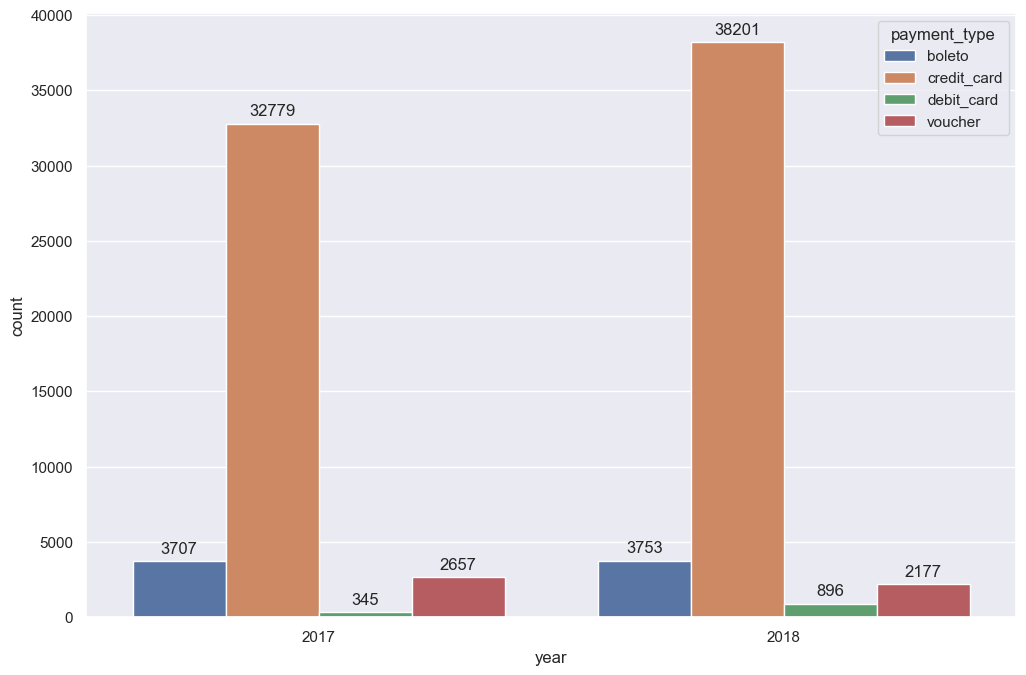
payment_count = orders_approval_hours.groupby(['payment_type', 'year']).size().reset_index(name='count')
payment_count
| payment_type | year | count | |
|---|---|---|---|
| 0 | boleto | 2017 | 3707 |
| 1 | boleto | 2018 | 3753 |
| 2 | credit_card | 2017 | 32779 |
| 3 | credit_card | 2018 | 38201 |
| 4 | debit_card | 2017 | 345 |
| 5 | debit_card | 2018 | 896 |
| 6 | voucher | 2017 | 2657 |
| 7 | voucher | 2018 | 2177 |
Majority of the payments were made through credit card. Credit card was also the fastest to be approved. Boleta takes around 5 hours to be approved, followed by more than 50 minutes in debit cards. In fact, more customers are using Boleto in 2018.
sns.set(style="darkgrid")
plt.figure(figsize=(12,8), dpi= 100)
splot = sns.barplot(x="year", y="count", hue="payment_type", data=payment_count, ci=None)
for p in splot.patches:
splot.annotate(format(p.get_height(), '.0f'),
(p.get_x() + p.get_width() / 2., p.get_height()),
ha = 'center', va = 'center',
xytext = (0, 9),
textcoords = 'offset points')
plt.show()
approve_deliver_proportion = delivered.copy(deep=False)
approve_deliver_proportion['deliver_days'] = (delivered['order_delivered_customer_date'] - delivered['order_approved_at']).dt.components['days']
approve_deliver_proportion = remove_outlier_iqr(approve_deliver_proportion, 'order_duration')
approve_deliver_proportion = remove_outlier_iqr(approve_deliver_proportion, 'deliver_days')
approve_deliver_proportion.head(3)
| order_id | customer_id | order_status | order_purchase_timestamp | order_approved_at | order_delivered_carrier_date | order_delivered_customer_date | order_estimated_delivery_date | order_delay | order_duration | year | approval_hours | deliver_days | |
|---|---|---|---|---|---|---|---|---|---|---|---|---|---|
| 0 | e481f51cbdc54678b7cc49136f2d6af7 | 9ef432eb6251297304e76186b10a928d | delivered | 2017-10-02 10:56:33 | 2017-10-02 11:07:15 | 2017-10-04 19:55:00 | 2017-10-10 21:25:13 | 2017-10-18 | -8.0 | 8.0 | 2017 | 0.0 | 8.0 |
| 1 | 53cdb2fc8bc7dce0b6741e2150273451 | b0830fb4747a6c6d20dea0b8c802d7ef | delivered | 2018-07-24 20:41:37 | 2018-07-26 03:24:27 | 2018-07-26 14:31:00 | 2018-08-07 15:27:45 | 2018-08-13 | -6.0 | 13.0 | 2018 | 6.0 | 12.0 |
| 2 | 47770eb9100c2d0c44946d9cf07ec65d | 41ce2a54c0b03bf3443c3d931a367089 | delivered | 2018-08-08 08:38:49 | 2018-08-08 08:55:23 | 2018-08-08 13:50:00 | 2018-08-17 18:06:29 | 2018-09-04 | -18.0 | 9.0 | 2018 | 0.0 | 9.0 |
approve_deliver_proportion['order_duration'].mean()
10.253967191161701
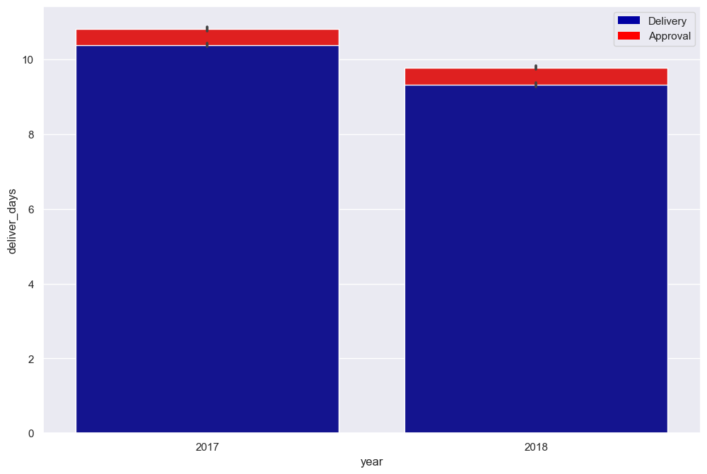
Although approval hours for payment method Boleto can take as much as 5 hours, majority of customer's waiting time goes into the delivery process.
sns.set(style="darkgrid")
plt.figure(figsize=(12,8), dpi= 100)
sns.barplot(x = approve_deliver_proportion['year'], y = approve_deliver_proportion['order_duration'], color = "red")
bottom_plot = sns.barplot(x = approve_deliver_proportion['year'], y = approve_deliver_proportion['deliver_days'], color = "#0000A3")
topbar = plt.Rectangle((0,0),1,1,fc="red", edgecolor = 'none')
bottombar = plt.Rectangle((0,0),1,1,fc='#0000A3', edgecolor = 'none')
l = plt.legend([bottombar, topbar], ['Delivery', 'Approval'])
products = pd.read_csv("olist_products_dataset.csv")
products.head(3)
| product_id | product_category_name | product_name_lenght | product_description_lenght | product_photos_qty | product_weight_g | product_length_cm | product_height_cm | product_width_cm | |
|---|---|---|---|---|---|---|---|---|---|
| 0 | 1e9e8ef04dbcff4541ed26657ea517e5 | perfumaria | 40.0 | 287.0 | 1.0 | 225.0 | 16.0 | 10.0 | 14.0 |
| 1 | 3aa071139cb16b67ca9e5dea641aaa2f | artes | 44.0 | 276.0 | 1.0 | 1000.0 | 30.0 | 18.0 | 20.0 |
| 2 | 96bd76ec8810374ed1b65e291975717f | esporte_lazer | 46.0 | 250.0 | 1.0 | 154.0 | 18.0 | 9.0 | 15.0 |
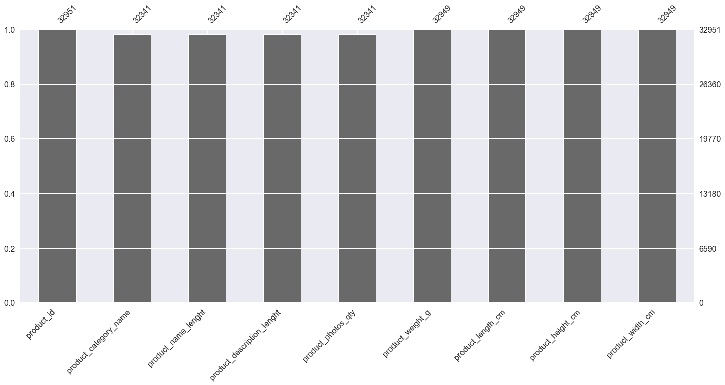
msno.bar(products)
<AxesSubplot:>
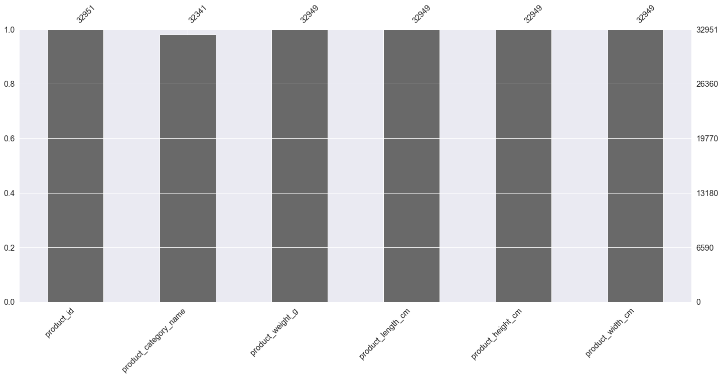
product_volume = products.drop(['product_description_lenght', 'product_photos_qty', 'product_name_lenght'], axis = 1)
msno.bar(product_volume)
<AxesSubplot:>
Translating product category name
category_translation = pd.read_csv("product_category_name_translation.csv")
category_translation.head(3)
| product_category_name | product_category_name_english | |
|---|---|---|
| 0 | beleza_saude | health_beauty |
| 1 | informatica_acessorios | computers_accessories |
| 2 | automotivo | auto |
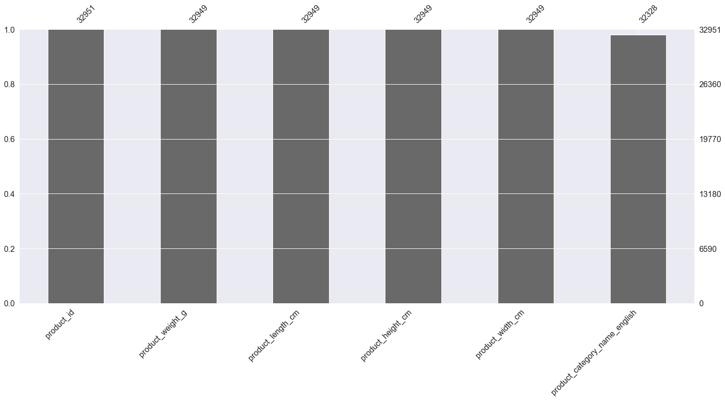
product_volume = pd.merge(product_volume, category_translation, how="left", on=["product_category_name"])
product_volume = product_volume.drop(['product_category_name'], axis = 1)
product_volume.head(3)
| product_id | product_weight_g | product_length_cm | product_height_cm | product_width_cm | product_category_name_english | |
|---|---|---|---|---|---|---|
| 0 | 1e9e8ef04dbcff4541ed26657ea517e5 | 225.0 | 16.0 | 10.0 | 14.0 | perfumery |
| 1 | 3aa071139cb16b67ca9e5dea641aaa2f | 1000.0 | 30.0 | 18.0 | 20.0 | art |
| 2 | 96bd76ec8810374ed1b65e291975717f | 154.0 | 18.0 | 9.0 | 15.0 | sports_leisure |
product_volume['product_category_name_english'].unique()
array(['perfumery', 'art', 'sports_leisure', 'baby', 'housewares',
'musical_instruments', 'cool_stuff', 'furniture_decor',
'home_appliances', 'toys', 'bed_bath_table',
'construction_tools_safety', 'computers_accessories',
'health_beauty', 'luggage_accessories', 'garden_tools',
'office_furniture', 'auto', 'electronics', 'fashion_shoes',
'telephony', 'stationery', 'fashion_bags_accessories', 'computers',
'home_construction', 'watches_gifts',
'construction_tools_construction', 'pet_shop', 'small_appliances',
'agro_industry_and_commerce', nan, 'furniture_living_room',
'signaling_and_security', 'air_conditioning', 'consoles_games',
'books_general_interest', 'costruction_tools_tools',
'fashion_underwear_beach', 'fashion_male_clothing',
'kitchen_dining_laundry_garden_furniture',
'industry_commerce_and_business', 'fixed_telephony',
'construction_tools_lights', 'books_technical',
'home_appliances_2', 'party_supplies', 'drinks', 'market_place',
'la_cuisine', 'costruction_tools_garden', 'fashio_female_clothing',
'home_confort', 'audio', 'food_drink', 'music', 'food',
'tablets_printing_image', 'books_imported',
'small_appliances_home_oven_and_coffee', 'fashion_sport',
'christmas_supplies', 'fashion_childrens_clothes', 'dvds_blu_ray',
'arts_and_craftmanship', 'furniture_bedroom', 'cine_photo',
'diapers_and_hygiene', 'flowers', 'home_comfort_2',
'security_and_services', 'furniture_mattress_and_upholstery',
'cds_dvds_musicals'], dtype=object)
There is no 'others' category, so for missing category names, they are considered 'others'
product_volume.fillna('others')
msno.bar(product_volume)
<AxesSubplot:>
product_volume['volume'] = product_volume['product_length_cm'] * product_volume['product_width_cm'] * product_volume['product_height_cm']
product_volume['weight'] = product_volume['product_weight_g'] / 1000
product_volume.head(3)
| product_id | product_weight_g | product_length_cm | product_height_cm | product_width_cm | product_category_name_english | volume | weight | |
|---|---|---|---|---|---|---|---|---|
| 0 | 1e9e8ef04dbcff4541ed26657ea517e5 | 225.0 | 16.0 | 10.0 | 14.0 | perfumery | 2240.0 | 0.225 |
| 1 | 3aa071139cb16b67ca9e5dea641aaa2f | 1000.0 | 30.0 | 18.0 | 20.0 | art | 10800.0 | 1.000 |
| 2 | 96bd76ec8810374ed1b65e291975717f | 154.0 | 18.0 | 9.0 | 15.0 | sports_leisure | 2430.0 | 0.154 |
product_volume.groupby('product_category_name_english').mean('volume').sort_values(by=['volume'], ascending=False)
| product_weight_g | product_length_cm | product_height_cm | product_width_cm | volume | weight | |
|---|---|---|---|---|---|---|
| product_category_name_english | ||||||
| furniture_mattress_and_upholstery | 13190.000000 | 46.300000 | 34.400000 | 41.300000 | 77244.300000 | 13.190000 |
| office_furniture | 12740.867314 | 55.627832 | 41.864078 | 37.919094 | 75468.469256 | 12.740867 |
| kitchen_dining_laundry_garden_furniture | 11598.563830 | 47.340426 | 40.478723 | 38.680851 | 69406.095745 | 11.598564 |
| home_appliances_2 | 9913.333333 | 45.733333 | 30.666667 | 38.166667 | 55476.311111 | 9.913333 |
| furniture_living_room | 8934.846154 | 50.730769 | 22.365385 | 44.429487 | 54486.128205 | 8.934846 |
| ... | ... | ... | ... | ... | ... | ... |
| watches_gifts | 509.287434 | 19.222724 | 10.292701 | 15.268623 | 3470.398044 | 0.509287 |
| books_technical | 1107.845528 | 27.325203 | 5.869919 | 18.463415 | 2758.991870 | 1.107846 |
| books_imported | 596.774194 | 29.741935 | 3.451613 | 21.225806 | 1935.387097 | 0.596774 |
| telephony | 236.506173 | 18.432981 | 6.853616 | 13.248677 | 1865.841270 | 0.236506 |
| dvds_blu_ray | 381.562500 | 21.270833 | 4.416667 | 14.875000 | 1746.854167 | 0.381562 |
71 rows × 6 columns
The heaviest and biggest product categories are furniture.
order_items.head(3)
| order_id | order_item_id | product_id | seller_id | shipping_limit_date | price | freight_value | |
|---|---|---|---|---|---|---|---|
| 0 | 00010242fe8c5a6d1ba2dd792cb16214 | 1 | 4244733e06e7ecb4970a6e2683c13e61 | 48436dade18ac8b2bce089ec2a041202 | 2017-09-19 09:45:35 | 58.9 | 13.29 |
| 1 | 00018f77f2f0320c557190d7a144bdd3 | 1 | e5f2d52b802189ee658865ca93d83a8f | dd7ddc04e1b6c2c614352b383efe2d36 | 2017-05-03 11:05:13 | 239.9 | 19.93 |
| 2 | 000229ec398224ef6ca0657da4fc703e | 1 | c777355d18b72b67abbeef9df44fd0fd | 5b51032eddd242adc84c38acab88f23d | 2018-01-18 14:48:30 | 199.0 | 17.87 |
order_weight_volume = pd.merge(delivered, order_items, how="left", on=["order_id"])
order_weight_volume = order_weight_volume.filter(['order_id', 'product_id'])
order_weight_volume.head(3)
| order_id | product_id | |
|---|---|---|
| 0 | e481f51cbdc54678b7cc49136f2d6af7 | 87285b34884572647811a353c7ac498a |
| 1 | 53cdb2fc8bc7dce0b6741e2150273451 | 595fac2a385ac33a80bd5114aec74eb8 |
| 2 | 47770eb9100c2d0c44946d9cf07ec65d | aa4383b373c6aca5d8797843e5594415 |
order_weight_volume = pd.merge(order_weight_volume, product_volume, how="left", on=["product_id"])
order_weight_volume = order_weight_volume.drop(columns=['product_weight_g', 'product_length_cm', 'product_width_cm', 'product_height_cm', 'product_id', 'product_category_name_english'])
order_weight_volume.head(3)
| order_id | volume | weight | |
|---|---|---|---|
| 0 | e481f51cbdc54678b7cc49136f2d6af7 | 1976.0 | 0.50 |
| 1 | 53cdb2fc8bc7dce0b6741e2150273451 | 4693.0 | 0.40 |
| 2 | 47770eb9100c2d0c44946d9cf07ec65d | 9576.0 | 0.42 |
order_weight_volume = order_weight_volume.groupby(['order_id']).sum(['volume', 'weight'])
order_weight_volume.head(3)
| volume | weight | |
|---|---|---|
| order_id | ||
| 00010242fe8c5a6d1ba2dd792cb16214 | 3528.0 | 0.65 |
| 00018f77f2f0320c557190d7a144bdd3 | 60000.0 | 30.00 |
| 000229ec398224ef6ca0657da4fc703e | 14157.0 | 3.05 |
order_weight_volume = pd.merge(order_weight_volume, delivered, how="left", on=["order_id"])
order_weight_volume.head(3)
| order_id | volume | weight | customer_id | order_status | order_purchase_timestamp | order_approved_at | order_delivered_carrier_date | order_delivered_customer_date | order_estimated_delivery_date | order_delay | order_duration | year | approval_hours | |
|---|---|---|---|---|---|---|---|---|---|---|---|---|---|---|
| 0 | 00010242fe8c5a6d1ba2dd792cb16214 | 3528.0 | 0.65 | 3ce436f183e68e07877b285a838db11a | delivered | 2017-09-13 08:59:02 | 2017-09-13 09:45:35 | 2017-09-19 18:34:16 | 2017-09-20 23:43:48 | 2017-09-29 | -9.0 | 7.0 | 2017 | 0.0 |
| 1 | 00018f77f2f0320c557190d7a144bdd3 | 60000.0 | 30.00 | f6dd3ec061db4e3987629fe6b26e5cce | delivered | 2017-04-26 10:53:06 | 2017-04-26 11:05:13 | 2017-05-04 14:35:00 | 2017-05-12 16:04:24 | 2017-05-15 | -3.0 | 16.0 | 2017 | 0.0 |
| 2 | 000229ec398224ef6ca0657da4fc703e | 14157.0 | 3.05 | 6489ae5e4333f3693df5ad4372dab6d3 | delivered | 2018-01-14 14:33:31 | 2018-01-14 14:48:30 | 2018-01-16 12:36:48 | 2018-01-22 13:19:16 | 2018-02-05 | -14.0 | 7.0 | 2018 | 0.0 |
class OrderWeightDashboard(param.Parameterized):
stats = param.ObjectSelector(default='volume', objects=['volume', 'weight'])
plt.figure(figsize=(12,8), dpi= 100)
def before_boxplot(self):
plt.clf()
sns.boxplot(x=order_weight_volume[self.stats])
return plt.gcf()
def after_boxplot(self):
plt.clf()
order_weight_volume_after = remove_outlier_iqr(order_weight_volume, self.stats)
sns.boxplot(x=order_weight_volume_after[self.stats])
return plt.gcf()
def append_end(self):
plt.clf()
return ""
ow1 = OrderWeightDashboard(name='')
dashboard = pn.Column('Order Weight Outlier Dashboard',
ow1.param,
pn.Tabs(
('Original', ow1.before_boxplot),
('Outlier removed', ow1.after_boxplot),
('',ow1.append_end)
)
)
dashboard.embed()
<Figure size 1728x1152 with 0 Axes>
order_weight_volume_corr = order_weight_volume.filter(['volume', 'weight', 'order_duration', 'approval_hours', 'order_delay', 'price', 'freight_value']).corr()
plt.figure(figsize=(12,8), dpi= 100)
sns.heatmap(order_weight_volume_corr, xticklabels=order_weight_volume_corr.columns, yticklabels=order_weight_volume_corr.columns, annot=True)
<AxesSubplot:>
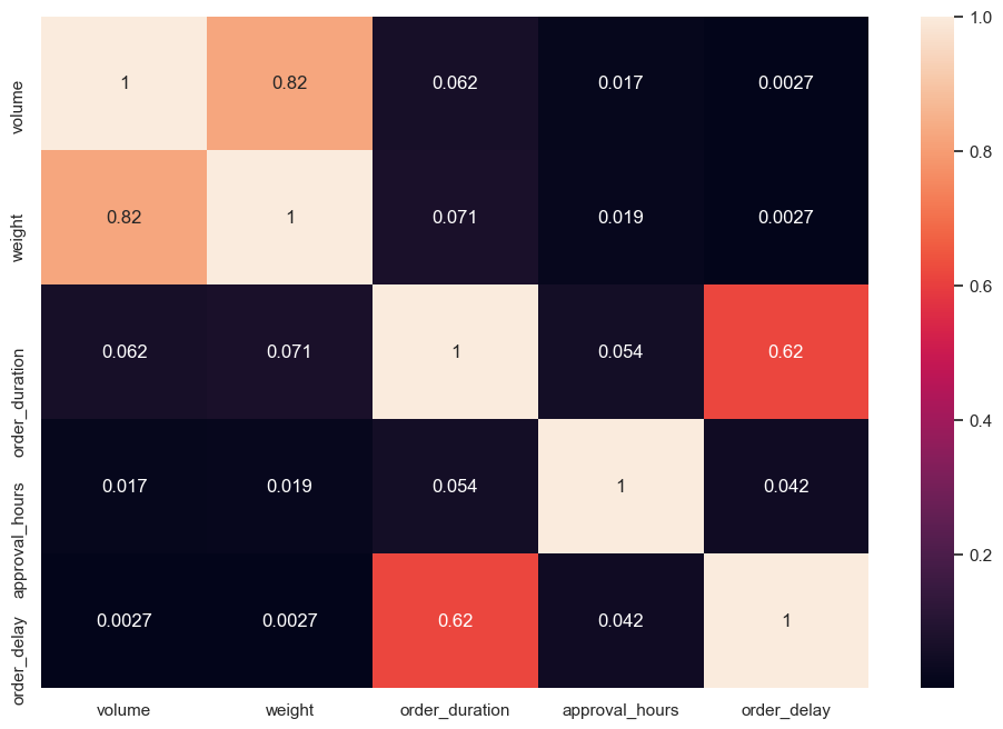
Order weight and volume are not correlated with order delivery.
geo = pd.read_csv("olist_geolocation_dataset.csv")
geo.head(3)
| geolocation_zip_code_prefix | geolocation_lat | geolocation_lng | geolocation_city | geolocation_state | |
|---|---|---|---|---|---|
| 0 | 1037 | -23.545621 | -46.639292 | sao paulo | SP |
| 1 | 1046 | -23.546081 | -46.644820 | sao paulo | SP |
| 2 | 1046 | -23.546129 | -46.642951 | sao paulo | SP |
avarage_location = geo.groupby('geolocation_state').mean(['geolocation_lat', 'geolocation_lng'])
avarage_location['geolocation_state'] = avarage_location.index
avarage_location.head(3)
| geolocation_zip_code_prefix | geolocation_lat | geolocation_lng | geolocation_state | |
|---|---|---|---|---|
| geolocation_state | ||||
| AC | 69798.877786 | -9.702555 | -68.451852 | AC |
| AL | 57234.456371 | -9.599729 | -36.052017 | AL |
| AM | 69142.245888 | -3.349336 | -60.537430 | AM |
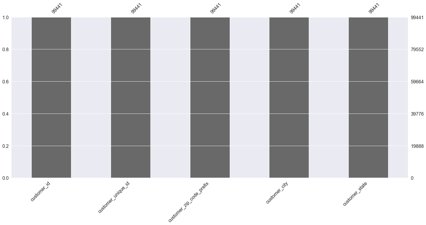
customers = pd.read_csv("olist_customers_dataset.csv")
customers.head(3)
| customer_id | customer_unique_id | customer_zip_code_prefix | customer_city | customer_state | |
|---|---|---|---|---|---|
| 0 | 06b8999e2fba1a1fbc88172c00ba8bc7 | 861eff4711a542e4b93843c6dd7febb0 | 14409 | franca | SP |
| 1 | 18955e83d337fd6b2def6b18a428ac77 | 290c77bc529b7ac935b93aa66c333dc3 | 9790 | sao bernardo do campo | SP |
| 2 | 4e7b3e00288586ebd08712fdd0374a03 | 060e732b5b29e8181a18229c7b0b2b5e | 1151 | sao paulo | SP |
msno.bar(customers)
<AxesSubplot:>
customer_state_geo = customers.merge(avarage_location.rename(columns={'geolocation_state':'customer_state'}),how='outer')
customer_state_geo.head(3)
| customer_id | customer_unique_id | customer_zip_code_prefix | customer_city | customer_state | geolocation_zip_code_prefix | geolocation_lat | geolocation_lng | |
|---|---|---|---|---|---|---|---|---|
| 0 | 06b8999e2fba1a1fbc88172c00ba8bc7 | 861eff4711a542e4b93843c6dd7febb0 | 14409 | franca | SP | 9054.286003 | -23.155308 | -47.084074 |
| 1 | 18955e83d337fd6b2def6b18a428ac77 | 290c77bc529b7ac935b93aa66c333dc3 | 9790 | sao bernardo do campo | SP | 9054.286003 | -23.155308 | -47.084074 |
| 2 | 4e7b3e00288586ebd08712fdd0374a03 | 060e732b5b29e8181a18229c7b0b2b5e | 1151 | sao paulo | SP | 9054.286003 | -23.155308 | -47.084074 |
import plotly.offline as pyo
import plotly.graph_objs as go
pyo.init_notebook_mode()
import plotly.express as px
fig = px.scatter_mapbox(customer_state_geo, lat="geolocation_lat", lon="geolocation_lng")
fig.update_layout(mapbox_style="open-street-map")
fig.show()
customer_state_density = avarage_location[avarage_location['geolocation_state'].isin(customer_state_geo['customer_state'])]
customer_state_density['count'] = customer_state_geo['customer_state'].value_counts()
customer_state_density
| geolocation_zip_code_prefix | geolocation_lat | geolocation_lng | geolocation_state | count | |
|---|---|---|---|---|---|
| geolocation_state | |||||
| AC | 69798.877786 | -9.702555 | -68.451852 | AC | 81 |
| AL | 57234.456371 | -9.599729 | -36.052017 | AL | 413 |
| AM | 69142.245888 | -3.349336 | -60.537430 | AM | 148 |
| AP | 68911.880422 | 0.086025 | -51.234304 | AP | 68 |
| BA | 44289.646858 | -13.049361 | -39.560649 | BA | 3380 |
| CE | 61662.827908 | -4.363151 | -39.004140 | CE | 1336 |
| DF | 71592.770137 | -15.810885 | -47.969630 | DF | 2140 |
| ES | 29327.859864 | -20.105145 | -40.503183 | ES | 2033 |
| GO | 75028.224440 | -16.577645 | -49.334195 | GO | 2020 |
| MA | 65411.114988 | -3.798997 | -44.818627 | MA | 747 |
| MG | 35354.955072 | -19.864647 | -44.421615 | MG | 11635 |
| MS | 79363.061068 | -20.765006 | -54.532140 | MS | 715 |
| MT | 78435.385670 | -14.156482 | -55.708956 | MT | 907 |
| PA | 67525.525569 | -2.631213 | -49.485862 | PA | 975 |
| PB | 58324.324305 | -7.088298 | -35.821678 | PB | 536 |
| PE | 53687.958678 | -8.179098 | -35.758866 | PE | 1652 |
| PI | 64324.879974 | -5.754989 | -42.509541 | PI | 495 |
| PR | 84328.662991 | -24.793607 | -50.879662 | PR | 5045 |
| RJ | 24002.060090 | -22.743477 | -43.155540 | RJ | 12852 |
| RN | 59280.773458 | -5.856702 | -35.990079 | RN | 485 |
| RO | 76885.564980 | -10.341289 | -62.720579 | RO | 253 |
| RR | 69315.043344 | 2.717100 | -60.672866 | RR | 46 |
| RS | 94996.301709 | -29.679191 | -52.032652 | RS | 5466 |
| SC | 88855.220492 | -27.222486 | -49.617937 | SC | 3637 |
| SE | 49197.524839 | -10.866199 | -37.181169 | SE | 350 |
| SP | 9054.286003 | -23.155308 | -47.084074 | SP | 41746 |
| TO | 77454.112975 | -9.503700 | -48.348661 | TO | 280 |
fig = px.density_mapbox(customer_state_density, lat='geolocation_lat', lon='geolocation_lng', z='count', radius=20,
center=dict(lat=0, lon=100), zoom=0,
mapbox_style="stamen-terrain")
fig.show()
Majority of the customers live in Sao Paulo.
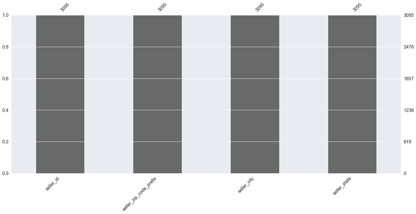
sellers = pd.read_csv("olist_sellers_dataset.csv")
sellers.head(3)
| seller_id | seller_zip_code_prefix | seller_city | seller_state | |
|---|---|---|---|---|
| 0 | 3442f8959a84dea7ee197c632cb2df15 | 13023 | campinas | SP |
| 1 | d1b65fc7debc3361ea86b5f14c68d2e2 | 13844 | mogi guacu | SP |
| 2 | ce3ad9de960102d0677a81f5d0bb7b2d | 20031 | rio de janeiro | RJ |
msno.bar(sellers)
<AxesSubplot:>
seller_state_geo = sellers.merge(avarage_location.rename(columns={'geolocation_state':'seller_state'}),how='outer')
seller_state_geo.head(3)
| seller_id | seller_zip_code_prefix | seller_city | seller_state | geolocation_zip_code_prefix | geolocation_lat | geolocation_lng | |
|---|---|---|---|---|---|---|---|
| 0 | 3442f8959a84dea7ee197c632cb2df15 | 13023.0 | campinas | SP | 9054.286003 | -23.155308 | -47.084074 |
| 1 | d1b65fc7debc3361ea86b5f14c68d2e2 | 13844.0 | mogi guacu | SP | 9054.286003 | -23.155308 | -47.084074 |
| 2 | c0f3eea2e14555b6faeea3dd58c1b1c3 | 4195.0 | sao paulo | SP | 9054.286003 | -23.155308 | -47.084074 |
fig = px.scatter_mapbox(seller_state_geo, lat="geolocation_lat", lon="geolocation_lng")
fig.update_layout(mapbox_style="open-street-map")
fig.show()
avarage_location
| geolocation_zip_code_prefix | geolocation_lat | geolocation_lng | geolocation_state | |
|---|---|---|---|---|
| geolocation_state | ||||
| AC | 69798.877786 | -9.702555 | -68.451852 | AC |
| AL | 57234.456371 | -9.599729 | -36.052017 | AL |
| AM | 69142.245888 | -3.349336 | -60.537430 | AM |
| AP | 68911.880422 | 0.086025 | -51.234304 | AP |
| BA | 44289.646858 | -13.049361 | -39.560649 | BA |
| CE | 61662.827908 | -4.363151 | -39.004140 | CE |
| DF | 71592.770137 | -15.810885 | -47.969630 | DF |
| ES | 29327.859864 | -20.105145 | -40.503183 | ES |
| GO | 75028.224440 | -16.577645 | -49.334195 | GO |
| MA | 65411.114988 | -3.798997 | -44.818627 | MA |
| MG | 35354.955072 | -19.864647 | -44.421615 | MG |
| MS | 79363.061068 | -20.765006 | -54.532140 | MS |
| MT | 78435.385670 | -14.156482 | -55.708956 | MT |
| PA | 67525.525569 | -2.631213 | -49.485862 | PA |
| PB | 58324.324305 | -7.088298 | -35.821678 | PB |
| PE | 53687.958678 | -8.179098 | -35.758866 | PE |
| PI | 64324.879974 | -5.754989 | -42.509541 | PI |
| PR | 84328.662991 | -24.793607 | -50.879662 | PR |
| RJ | 24002.060090 | -22.743477 | -43.155540 | RJ |
| RN | 59280.773458 | -5.856702 | -35.990079 | RN |
| RO | 76885.564980 | -10.341289 | -62.720579 | RO |
| RR | 69315.043344 | 2.717100 | -60.672866 | RR |
| RS | 94996.301709 | -29.679191 | -52.032652 | RS |
| SC | 88855.220492 | -27.222486 | -49.617937 | SC |
| SE | 49197.524839 | -10.866199 | -37.181169 | SE |
| SP | 9054.286003 | -23.155308 | -47.084074 | SP |
| TO | 77454.112975 | -9.503700 | -48.348661 | TO |
seller_state_density = avarage_location[avarage_location['geolocation_state'].isin(seller_state_geo['seller_state'])]
seller_state_density['count'] = seller_state_geo['seller_state'].value_counts()
seller_state_density
| geolocation_zip_code_prefix | geolocation_lat | geolocation_lng | geolocation_state | count | |
|---|---|---|---|---|---|
| geolocation_state | |||||
| AC | 69798.877786 | -9.702555 | -68.451852 | AC | 1 |
| AL | 57234.456371 | -9.599729 | -36.052017 | AL | 1 |
| AM | 69142.245888 | -3.349336 | -60.537430 | AM | 1 |
| AP | 68911.880422 | 0.086025 | -51.234304 | AP | 1 |
| BA | 44289.646858 | -13.049361 | -39.560649 | BA | 19 |
| CE | 61662.827908 | -4.363151 | -39.004140 | CE | 13 |
| DF | 71592.770137 | -15.810885 | -47.969630 | DF | 30 |
| ES | 29327.859864 | -20.105145 | -40.503183 | ES | 23 |
| GO | 75028.224440 | -16.577645 | -49.334195 | GO | 40 |
| MA | 65411.114988 | -3.798997 | -44.818627 | MA | 1 |
| MG | 35354.955072 | -19.864647 | -44.421615 | MG | 244 |
| MS | 79363.061068 | -20.765006 | -54.532140 | MS | 5 |
| MT | 78435.385670 | -14.156482 | -55.708956 | MT | 4 |
| PA | 67525.525569 | -2.631213 | -49.485862 | PA | 1 |
| PB | 58324.324305 | -7.088298 | -35.821678 | PB | 6 |
| PE | 53687.958678 | -8.179098 | -35.758866 | PE | 9 |
| PI | 64324.879974 | -5.754989 | -42.509541 | PI | 1 |
| PR | 84328.662991 | -24.793607 | -50.879662 | PR | 349 |
| RJ | 24002.060090 | -22.743477 | -43.155540 | RJ | 171 |
| RN | 59280.773458 | -5.856702 | -35.990079 | RN | 5 |
| RO | 76885.564980 | -10.341289 | -62.720579 | RO | 2 |
| RR | 69315.043344 | 2.717100 | -60.672866 | RR | 1 |
| RS | 94996.301709 | -29.679191 | -52.032652 | RS | 129 |
| SC | 88855.220492 | -27.222486 | -49.617937 | SC | 190 |
| SE | 49197.524839 | -10.866199 | -37.181169 | SE | 2 |
| SP | 9054.286003 | -23.155308 | -47.084074 | SP | 1849 |
| TO | 77454.112975 | -9.503700 | -48.348661 | TO | 1 |
fig = px.density_mapbox(seller_state_density, lat='geolocation_lat', lon='geolocation_lng', z='count', radius=20,
center=dict(lat=0, lon=100), zoom=0,
mapbox_style="stamen-terrain")
fig.show()
Majority of the sellers also live in Sao Paulo
from math import sin, cos, sqrt, atan2, radians
def get_distance(lat1, lat2, lon1, lon2):
# approximate radius of earth in km
R = 6373.0
dlon = lon2 - lon1
dlat = lat2 - lat1
a = sin(dlat / 2)**2 + cos(lat1) * cos(lat2) * sin(dlon / 2)**2
c = 2 * atan2(sqrt(a), sqrt(1 - a))
return(R * c)
Customized function to get distance between 2 coordinates
order_distance = pd.merge(delivered, customer_state_geo.filter(['customer_id', 'geolocation_lat', 'geolocation_lng']), how="left", on=["customer_id"])
order_distance = order_distance.rename(columns={'geolocation_lat': 'customer_lat', 'geolocation_lng': 'customer_lng'})
order_distance.head(3)
| order_id | customer_id | order_status | order_purchase_timestamp | order_approved_at | order_delivered_carrier_date | order_delivered_customer_date | order_estimated_delivery_date | order_delay | order_duration | year | approval_hours | customer_lat | customer_lng | |
|---|---|---|---|---|---|---|---|---|---|---|---|---|---|---|
| 0 | e481f51cbdc54678b7cc49136f2d6af7 | 9ef432eb6251297304e76186b10a928d | delivered | 2017-10-02 10:56:33 | 2017-10-02 11:07:15 | 2017-10-04 19:55:00 | 2017-10-10 21:25:13 | 2017-10-18 | -8.0 | 8.0 | 2017 | 0.0 | -23.155308 | -47.084074 |
| 1 | 53cdb2fc8bc7dce0b6741e2150273451 | b0830fb4747a6c6d20dea0b8c802d7ef | delivered | 2018-07-24 20:41:37 | 2018-07-26 03:24:27 | 2018-07-26 14:31:00 | 2018-08-07 15:27:45 | 2018-08-13 | -6.0 | 13.0 | 2018 | 6.0 | -13.049361 | -39.560649 |
| 2 | 47770eb9100c2d0c44946d9cf07ec65d | 41ce2a54c0b03bf3443c3d931a367089 | delivered | 2018-08-08 08:38:49 | 2018-08-08 08:55:23 | 2018-08-08 13:50:00 | 2018-08-17 18:06:29 | 2018-09-04 | -18.0 | 9.0 | 2018 | 0.0 | -16.577645 | -49.334195 |
order_distance = pd.merge(order_distance, order_items.filter(['order_id', 'seller_id']), how="left", on=["order_id"])
order_distance = pd.merge(order_distance, seller_state_geo.filter(['seller_id', 'geolocation_lat', 'geolocation_lng']), how="left", on=["seller_id"])
order_distance = order_distance.rename(columns={'geolocation_lat': 'seller_lat', 'geolocation_lng': 'seller_lng'})
order_distance.head(3)
| order_id | customer_id | order_status | order_purchase_timestamp | order_approved_at | order_delivered_carrier_date | order_delivered_customer_date | order_estimated_delivery_date | order_delay | order_duration | year | approval_hours | customer_lat | customer_lng | seller_id | seller_lat | seller_lng | |
|---|---|---|---|---|---|---|---|---|---|---|---|---|---|---|---|---|---|
| 0 | e481f51cbdc54678b7cc49136f2d6af7 | 9ef432eb6251297304e76186b10a928d | delivered | 2017-10-02 10:56:33 | 2017-10-02 11:07:15 | 2017-10-04 19:55:00 | 2017-10-10 21:25:13 | 2017-10-18 | -8.0 | 8.0 | 2017 | 0.0 | -23.155308 | -47.084074 | 3504c0cb71d7fa48d967e0e4c94d59d9 | -23.155308 | -47.084074 |
| 1 | 53cdb2fc8bc7dce0b6741e2150273451 | b0830fb4747a6c6d20dea0b8c802d7ef | delivered | 2018-07-24 20:41:37 | 2018-07-26 03:24:27 | 2018-07-26 14:31:00 | 2018-08-07 15:27:45 | 2018-08-13 | -6.0 | 13.0 | 2018 | 6.0 | -13.049361 | -39.560649 | 289cdb325fb7e7f891c38608bf9e0962 | -23.155308 | -47.084074 |
| 2 | 47770eb9100c2d0c44946d9cf07ec65d | 41ce2a54c0b03bf3443c3d931a367089 | delivered | 2018-08-08 08:38:49 | 2018-08-08 08:55:23 | 2018-08-08 13:50:00 | 2018-08-17 18:06:29 | 2018-09-04 | -18.0 | 9.0 | 2018 | 0.0 | -16.577645 | -49.334195 | 4869f7a5dfa277a7dca6462dcf3b52b2 | -23.155308 | -47.084074 |
order_distance['order_distance'] = order_distance.apply(lambda x: get_distance(x['customer_lat'], x['customer_lng'], x['seller_lat'], x['seller_lng']), axis=1)
order_distance.head(3)
| order_id | customer_id | order_status | order_purchase_timestamp | order_approved_at | order_delivered_carrier_date | order_delivered_customer_date | order_estimated_delivery_date | order_delay | order_duration | year | approval_hours | customer_lat | customer_lng | seller_id | seller_lat | seller_lng | order_distance | |
|---|---|---|---|---|---|---|---|---|---|---|---|---|---|---|---|---|---|---|
| 0 | e481f51cbdc54678b7cc49136f2d6af7 | 9ef432eb6251297304e76186b10a928d | delivered | 2017-10-02 10:56:33 | 2017-10-02 11:07:15 | 2017-10-04 19:55:00 | 2017-10-10 21:25:13 | 2017-10-18 | -8.0 | 8.0 | 2017 | 0.0 | -23.155308 | -47.084074 | 3504c0cb71d7fa48d967e0e4c94d59d9 | -23.155308 | -47.084074 | 9339.120177 |
| 1 | 53cdb2fc8bc7dce0b6741e2150273451 | b0830fb4747a6c6d20dea0b8c802d7ef | delivered | 2018-07-24 20:41:37 | 2018-07-26 03:24:27 | 2018-07-26 14:31:00 | 2018-08-07 15:27:45 | 2018-08-13 | -6.0 | 13.0 | 2018 | 6.0 | -13.049361 | -39.560649 | 289cdb325fb7e7f891c38608bf9e0962 | -23.155308 | -47.084074 | 7705.414246 |
| 2 | 47770eb9100c2d0c44946d9cf07ec65d | 41ce2a54c0b03bf3443c3d931a367089 | delivered | 2018-08-08 08:38:49 | 2018-08-08 08:55:23 | 2018-08-08 13:50:00 | 2018-08-17 18:06:29 | 2018-09-04 | -18.0 | 9.0 | 2018 | 0.0 | -16.577645 | -49.334195 | 4869f7a5dfa277a7dca6462dcf3b52b2 | -23.155308 | -47.084074 | 6855.903768 |
class OrderDistanceDashboard(param.Parameterized):
stats = param.ObjectSelector(default='Original', objects=['Original', 'Outlier removed'])
plt.figure(figsize=(12,8), dpi= 100)
def after_boxplot(self):
plt.clf()
if self.stats == 'Original':
sns.boxplot(x=order_distance['order_distance'])
else:
order_no_outlier = remove_outlier_iqr(order_distance, 'order_distance')
sns.boxplot(x=order_no_outlier['order_distance'])
return plt.gcf()
def append_end(self):
plt.clf()
return ""
od1 = OrderPriceDashboard(name='')
dashboard = pn.Column('Order Distance Outlier Dashboard',
od1.param,
od1.after_boxplot,
od1.append_end
)
dashboard.embed()
<Figure size 1728x1152 with 0 Axes>
order_distance_corr = order_distance.filter(['order_distance', 'order_duration', 'approval_hours', 'order_delay']).corr()
plt.figure(figsize=(12,8), dpi= 100)
sns.heatmap(order_distance_corr, xticklabels=order_distance_corr.columns, yticklabels=order_distance_corr.columns, annot=True)
<AxesSubplot:>
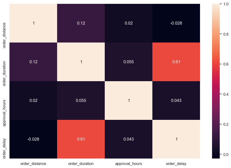
Distance is not a reliable predictor for delivery time taken